The City’s Advanced Stats Primer

I’m putting together this advanced stats primer for GSOM. Figured I post it here and solicit input from the more specialized crowd that frequents my personal blog. Most of  you know this stuff, but it never hurts to hear it from someone who might have a slightly different take. Any comments are welcome, except those I don’t like. 😛

APBR

Association for Professional Basketball Research – like their SABRmetric baseball counterparts, advanced basketball stat gurus are often called APBRmetricians. Just thought you should know the acronym in case you come across it. There’s a dedicated APBR forum for many years now that has played host to numerous debates in the community, and it’s interesting to note that many of the forum members eventually went on to work for NBA teams (Dean Oliver) or ESPN (John Hollinger). Yours truly posts there from time to time.

Shooting Stats

eFG%: Effective Field Goal Percentage

eFG% = 100 * (FG + 0.5*3PT) / FGA

The formula says you take the number of field goals (FG) a player makes, add to that half the number of 3pt field goals made (3PT), then divide by the total number of field goal attempts (FGA). If a player never takes any 3pt shots, then his eFG% will be equal to the usual FG% (100*FG/FGA). If a player only takes 3pt shots, then his eFG% is equal to 1.5 times his FG% (let’s ignore the fact that in theory the highest possible eFG% is actually greater than 100%). Obviously, most players fall somewhere in between these two extremes. The idea behind eFG% is that it takes into account (and rewards) players for making shots that are worth more (i.e. 3pt shots). Note that there is no “extra” penalty for missing a 3pt shot. In other words, all missed shots are worth the same amount. According to Basketball-Reference, DeAndre Jordan led the league in eFG% this past season (68.6%). Reggie Williams finished 20th (55.8%) and Stephen Curry finished 24th (55.1%). The league average eFG% last season was just about 50%. Note that eFG% can be applied equally to players or teams.

Sources: Basketball-Reference, 82games

TS%: True shooting percentage

TS% = 100 * (1/2) * PTS / (FGA + 0.44*FTA)

Among the advanced shooting stats, perhaps, none gets thrown around as much as TS%. The idea behind this stat is that it takes into account *all* the points a player gets via field goal shooting and foul shooting (which is not accounted for by FG% or eFG%). Given that the ratio of FTA/FGA last season was just about 30%, you can see why it would matter. In fact many of the best players in the league heavily rely on foul shooting to amass their points. And because free throws are so much easier to make than field goals, these players tend to get points more easily (i.e. more efficiently). Therefore, users of advanced stats tend to like TS% moreso than FG% or eFG% when talking about a player’s shooting efficiency.

Let’s talk a bit more about the formula. We want to know how efficient a player is in terms of scoring points per shot taken. If we forget about free throws for a minute, then the formula becomes PTS/(2*FGA), which happens to be equivalent to eFG%. Now let’s think about foul shots. The box score doesn’t tell us how many shots a player was fouled on. It just tells us how many foul shots were taken and made. Fortunately, smart folks many years ago figured out that, on average, the equivalent number of shots taken by a player is 0.44 times the number of FTA taken. By using play-by-play data, instead of box scores, it’s actually possible to determine exactly how many equivalent shots were taken by each player, but I don’t know of any source that publishes or calculates those stats (not exactly, anyway). Last season, Tyson Chandler led the league in TS% (69.7%) according to Basketball-Reference. Like eFG%, TS% can be applied to players or teams. The league average TS% was about 54% last season.

Sources: Basketball-Reference, Hoopdata

PPP: Points Per Possession (alternatively Points Per Play)

PPP = PTS/POSS

PPP is a shooting stat that is deceptively simple. It describes how efficiently a player scores with the possessions that he uses. If you think about it, there are a limited number of possessions in a game, and only 1 of 5 players can take a shot each time down the floor. Ideally, you’d like to make sure your most efficient players take the most efficient shots. PPP is what we most often use to do this analysis. In order to utilize it, obviously, we first need to know how to count possessions. More specifically, we need to define possessions used by a player in a way that can be calculated using box score stats (i.e. unfortunately, there is no box score stat called “possessions”). The generally accepted (and simplest) “box score” definition is:

POSS = FGA + 0.44*FTA + TOV

In other words, an (offensive) possession used includes field goal attempts, free throws, and turnovers. Note that it doesn’t account for possessions that a player creates through rebounding or steals, although as we will see later, there are other stats that do so. PPP is used quite a bit in advanced stats circles these days, perhaps, due to the popularity of Synergy (explained later). By my own calculations (based on play-by-play data), Tyson Chandler led the league last season with a 1.21 PPP. Reggie Williams led the Warriors with 1.08 PPP and Curry came in 2nd at 1.01 (lower due to turnovers). Obviously, guards will generally have lower PPP, because they tend to produce more TOV. One should be aware of that when citing PPP.

Sources: Synergy (and me)

PSAMS (Position- and Shot-Adjusted Marginal Scoring)

This is a shooting stat that I recently developed, and will use from time to time. As the name suggests, it takes into account both the position and type of shot (inside, mid-range, 3pt, free throw). Unlike a lot of other shooting stats, it also tries to account for volume by comparing how many shots a player takes of each type relative to the average player at his same position. Dirk Nowitzki had the highest total PSAMS rating in 2011, followed by LeBron James, Kevin Martin, Kevin Durant, and Paul Pierce. It can be applied at the team level, in addition to the player level, and also can be used on defense. Here are links to the original articles describing each component of the metric:

PSAMS: Inside Shots

PSAMS: Mid-Range Shots

PSAMS: 3pt Shots

PSAMS: Foul Shots

PSAMS: Total Scoring

The most recent PSAMS ratings for the current season can always be found here.

Pace- and Volume-Adjusted Stats (alternatively called “Tempo-Free”)

REB%, AST%, BLK%, STL%, TOV%, USG%

Instead of citing rebounds per game, assists per game, etc, advanced stats followers typically use these pace- and volume-adjusted stats which frame the stat as a percentage. Given that pace is defined as the number of team possessions per 48 minutes, it should be obvious that pace varies between teams, sometimes by quite a lot. Last season, Minnesota led the league with a 96.5 pace, while Portland had the slowest pace at 87.9. Teams that play at a faster pace are generally going to have inflated per-game and per-minute stats, which may make a player appear better (or worse!) than he would be after taking into account pace. The reason for volume adjustment is that different players play different amounts of minutes. For example, all else being equal, a player who plays 40 mpg is going to amass more per-game stats than a player with the same ability who plays 32 mpg. By using %’s (as defined below), we kill two birds with one stone by adjusting for pace and minutes (volume) played.

• REB% is the number of rebounds a player gets divided by the total number of rebounding opportunities (x100).
• AST% is an estimate of the percentage of shots a player assisted his teammates on. (This is not to be confused with %AST, which is the percentage of shots a player takes that are assisted!)
• BLK% is the percentage of opponent shots that a player blocks.
• STL% is the ratio of a player’s steals to the total number of opponent possessions expressed as a percentage.
• TOV% is similarly the ratio of a player’s TOV to his own team’s possessions expressed as a percentage.
• USG% is the percentage of team possessions (POSS) that a player uses either through shots attempts, turnovers, or getting fouled (FGA+TOV+0.44*FTA). So, it’s USG%=100*(FGA+TOV+0.44*FTA)/POSS. Some also count a fraction of the assists that a player gets (e.g. 0.3*AST) in the numerator.

Please note, using these pace- and volume-adjusted stats will make you a better person.

Sources: Basketball-Reference

Measures of Team Strength

ORTG, DRTG

ORTG = 100*(PTS Scored)/POSS
DRTG = 100*(PTS Allowed)/POSS

Arguably, the two most important stats in basketball (aside from wins) are the offensive rating (ORTG) and defensive rating (DRTG). Instead of citing points scored per game or points allowed per game, we adjust for the pace of each team, by dividing the total points scored (allowed) by the total number of possessions and then multiply by 100. The average ORTG and DRTG last season was 107.3. Obviously, better teams tend to have higher ORTG and lower DRTG.

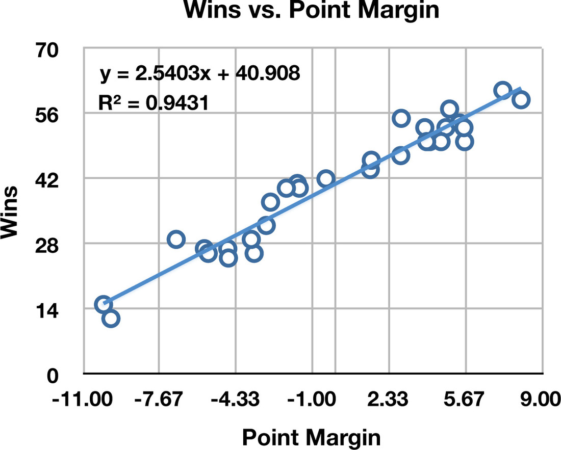
It turns out that the difference between ORTG and DRTG (point margin per 100 possessions) correlates extremely well with winning. I wrote it about here. Here it is depicted graphically:

via thecity2.files.wordpress.com

That plot was made using team wins from the 2009-10 season. The formula for (expected) wins is:

Wins = 2.54*PM + 41

For example, last season GSW had an 108.2 ORTG and 110.7 DRTG, the difference of which is -2.5 (ORTG-DRTG). Putting that in the formula gives 2.54*(-2.5)+41 = 34.65 ~ 35 wins. The Warriors actually won 36 games, a difference of only 1 game from what would be expected given their ORTG and DRTG. Pretty neat, eh?

Sources: Basketball-Reference, Hoopdata

Four Factors (eFG%, TOV%, FTA/FGA, REB%)

Dean Oliver, who formerly worked as “the stats guy” for Denver and now works at ESPN (in fact, he’s one of the main guys responsible for coming up with QBR, for better or worse, depending on your viewpoint), wrote in his book Basketball on Paper (a must read in my opinion):

There are four factors of an offense or defense that define its efficiency: shooting percentage, turnover rate, offensive rebounding percentage, and getting to the foul line. Striving to control those factors leads to a more successful team.

Here is a post Oliver wrote on the subject in 2004. I wrote two articles on the correlation between these four factors (often simply abbreviated “FF”) and team wins (Part 1 and Part 2). It turns out that these four factors (well, 8 factors, if you consider offense and defense, of course) account for a whopping 96% of point differential. (For the technical details consult Part 1 of that series.) Moreover, of the four factors, I estimated that eFG% accounts for about 54% (40%) of the total, turnovers account for 22% (25%), rebounding 15% (20%), and foul rate 10% (15%). The numbers in parentheses refer to the values that Oliver found. I’m not sure exactly how he arrived at his weights, but you can see they are on the same order as mine. The details of my analysis are given in Part 2. The significance of all this is that it’s really, really, really, really, really (really) important for your team to shoot well and defend the shot well. It’s really, really important to take care of the ball and force turnovers. It’s really important to rebound. It’s important to draw fouls and not foul the opponent too much, too. Everything else you can think of on a basketball court, if it’s not related to one of these things, is probably not that big of a deal.

(BTW, see how the number of “really”s was correlated to the importance? Ok, good. Just checking.)

Sources: Basketball-Reference, hoopdata

Synergy

Synergy is a commercial service that analyzes game film and calculates offensive and defensive PPP (see above) according to different play categories, including:

• isolation
• pick-and-roll – ball handler
• pick-and-roll – man
• spot-up
• off-screen
• hand-off
• transition
• cut to the basket
• offensive rebound (e.g. tip)

I’ve written numerous articles featuring Synergy stats. Here’s a summary of the 2010-11 season according to Synergy, and here’s a post on the value of each shot type. In addition to the team level data, Synergy also provides data for individual players in the same categories. You can do neat stuff with Synergy. For example, here is a treemap that summarizes the Synergy stats for a GSW-SAS game (size of tiles refers to fraction of points scored by that shot type and color refers to PPP with red being higher):

Synergy stats for a GSW-SAS game.

Sources: Synergy

“One Number” Measures of Player Productivity

The idea behind these stats is that they boil down all of a player’s value to one number. In some cases, the number can be put in terms of wins a player contributes to his team. I’ll briefly discuss some of the most frequently used metrics, but the provided links should be followed to get the full details. All the metrics in this list are considered “linear weights” metrics, as they are (not surprisingly) a linearly weighted sum of the various statistical categories (i.e. rebounds, field goals, assists, etc.). The weights or coefficients are found either by regression or “theory”.

In one way or another, each of these metrics places relative value on each statistical category according to the value of a possession, which is around 1.08 PPP. For example, a 2-pt shot is worth (2-1.08) = 0.92 PPP. A 3-pt shot would be worth 1.92 PPP. A steal results in a gain of a possession, which is worth 1.08 PPP. Therefore, a linear weight metric might give a player 0.92 pts for each 2-pt field goal made, 1.92 points for each 3-pt bucket, and 1.08 points for each steal. All the metrics generally agree on these values. Where the major differences arise usually revolves around the value (or penalty) given for missing shots and for rebounds (both offensive and defensive).

PER

PER stands for Player Efficiency Rating (click on the link to see the formula) and was developed by John Hollinger (ESPN). Although a lot of people these days tend to criticize Hollinger, it should be noted that he is one of the most influential of the early APBRmetricians and is still well-respected in that community. There are several common criticisms of PER: 1) It does not account for defense, except for blocks and defensive rebounds; 2) It tends to reward high-volume, low-efficiency scorers; and 3) It is not useful as a predictive tool.

sources: ESPN (Insider)

Win Shares (WS)

WS is calculated by the folks at Basketball-Reference (see link for more details) and is based on the formulas detailed in Dean Oliver’s Basketball on Paper (if you have any interest in getting into the world of advanced stats, do yourself a favor and head straight to Amazon and buy the book). Like PER, WS is based solely on box score statistics. Unlike PER, it does attempt to account for defense, although it’s a fairly rough estimate given the lack of defensive data available from the box score. If you add up all the WS for players on a team, it should roughly equal the total wins for that team during the course of a season. One thing about WS that’s nice is that it’s fairly non-controversial compared to PER or WP. Also, it’s arguably the most accessible of all the box score metrics, given the popularity and ease-of-use of the B-R website.

sources: Basketball-Reference

Wins Produced (WP)

WP is the metric developed (and popularized) by David Berri and colleagues several years ago that was detailed (more or less) in the book Wages of Wins. Berri also runs a website featuring WP-based analyses. Unfortunately, there is a long-running feud (or maybe cold war is the best way to say it) between Berri and his “followers” and most of the rest of the APBRmetricians in the universe. Like WS, WP is a box score metric. The two main problems that people tend to cite about WP are that it places too much value on rebounding and shooting efficiency. It’s impossible to re-hash all the arguments that have taken place on these fronts, but if you read my original ezPM article, you probably can get the gist of it. Here’s another article by Phil Birnbaum on the subject of rebounding.

sources: Wages of Wins blog

ezPM

This is my baby. Basically, I spent the winter of 2010 thinking about basketball statistics and how I might come up with an improvement on WP (and WS and PER, to be honest). The main innovation I came up with was to use play-by-play data (which enables me to know all the specific units being used on every possession) and counterpart data for better handling of defense. I’ve spent a lot of time on ezPM, but it’s certainly not perfect. In fact, these days I tend to favor one of the +/- flavors (RAPM) discussed later on for serious analysis. One advantage of ezPM, however, is that you can use it in short series (playoffs) or a small subset of games where the sample size is not going to be large enough for reliable +/- statistics. It should be noted, however, and in defense of ezPM, that it actually performs pretty well as a predictor (better than WP, but not quite as good as RAPM) in the only rigorous study I know of that’s compared all three metrics. If you’re interested in those articles (by Alex Konkel) see here.

ezPM ratings for all players can be found here, for rookies here, for sophomores here, and for non-starters (“6th men”) here.

sources: The City

Expected Value (EV)

EV is a really cool metric that is similar in many ways to ezPM, except that the guy who created it (“ElGee”) actually uses video to do his stat tracking. That way he can record things like “defensive errors” and “opportunities created”. It’s really neat stuff, and I highly recommend following ElGee’s work on it. The main issue I have is not with the details of the metric itself, but simply the fact that it’s not very high-throughput at this point or repeatable by others, since it’s all done by ElGee essentially by hand. Of the 1230 games in a season (990 this season), he watches a relatively small sample (as far as I know). At any rate, the logic of EV is sound in my opinion.

sources: Backpicks

Plus-Minus (+/-)

This family of stats is so ubiquitous now, I think it deserves its own category.

First, what is +/-? At the team level, this is the number of points a team (or specific unit) goes up or falls behind while it is on the floor. If starters played an entire game, this would simply be the point differential at the end of the game. Because players come in and out of the game (and thus, there are many different units), +/- typically refers to the number of points a team goes up or down while a player was in the game. In other words, +/- is assigned to individual players, but represents a team outcome. If Stephen Curry’s +/- is +10 in a game, that doesn’t (necessarily) mean Curry created a +10 point differential by himself. All it means is that while Curry was on the floor, the Warriors outscored their opponent by 10 points. (Another way to think about this is that the ORTG-DRTG for the team while the player was on the floor is +10.) Therefore, to be a meaningful statistic for evaluating players, what we really want to know is the individual +/-, or how a particular player contributed to the aggregate +/-. Say Curry was +5, Ellis was +6, Lee was +2, Biedrins was +1 and Dorell Wright was -4. In this example, the team +/- is +10, but Dorell Wright was actually a negative contributer. Going a step further, we can foresee a situation where some players are attributed +/- stats simply by playing with 4 other really good players.

To make it more clear which type of +/- we are talking about, I (and others) typically refer to the aggregate or team +/- as the “unadjusted +/-“. The individual +/- (attributed to the player independent of his teammates) is called the “adjusted +/-“, because we need to adjust for the quality of his teammates and opponents while he was on the floor. If you see the term APM being used, it refers to “adjusted +/-“.

Ok, so the big question is how do we get from the unadjusted +/- to the APM? The short technical answer is we use some form of linear regression. Eli Witus (who used to be an APBR forum member before he got a job working for the Houston Rockets) wrote a great article a few years ago on how to calculate APM. I’m going to try to give a high-level overview of the strategy (see Witus’ article for the nitty gritty details and implementation).

I’m going to use football as a starting point. Imagine we want to know the strength (power rating) of every NFL team. The reason we want to know such a thing is so that we can predict the result when two teams face each other. To do this, we first assume that each team can be described by a single rating. This sounds obvious, but what it means is that regardless of the matchup, we can always use the same rating for each team. This is the assumption of linearity. An alternative non-linear assumption would be that teams have different ratings versus different teams. It’s not that the latter assumption is technically wrong; however, given the limited amount of data (i.e. games) in a single season, it is not a practical solution. Therefore, we stick with the linear assumption and assume that each team has a single rating. Given our assumption, let’s say that San Francisco is hosting Arizona and we want to predict the outcome:

MOV = HFA + SF - ARI = 3.0 + 5.0 - 3.5 = 4.5

This equation says the margin of victory (MOV) is equal to the home field advantage (usually around 3 pts) + San Francisco’s rating (which is close to roughly 5 at the time I’m writing this) minus Arizona’s current rating (roughly -3.5). In this case, the equation tells us that the predicted outcome is SF winning by 4.5 points.

But how do we get those ratings? Basically, we reverse the process mathematically and use the actual results from previous games. For example, in the recent “Harbowl”, Baltimore beat SF 16-6:

10 = HFA + BAL - SF

See, now we know the MOV from that game, but we don’t know any of the three values. We can set up an equation like this for every game that has been played. Once we’ve done that, we then use linear regression to calculate for us what the ratings were that most closely replicate the data for each game. Of course, there is a lot of error involved. It’s obvious that for each game, the results are not going to go exactly according to the ratings. Sometimes, the higher rated team loses, after all. However, on average, the weights/ratings determined from the regression give us the lowest error out of all the possible linear weights we could imagine. This is often called BLUE (best linear unbiased estimate).

We need to take one final step to bring it back to basketball and calculating player ratings. Essentially, we set up the same equations, but instead of using the results from games, we use the results from each possession of a game. Instead of margin of victory, we use the point differential over a series of possessions played while two opposing 5-man units were on the floor. Here’s an actual example of a 9-possession stint (series of possessions in two units face each other before a substitution is made) during a GSW-NOH game at Oracle Arena last season:

-8 = HCA + (Curry + Ellis + D. Wright + Lee + Biedrins) 
- (Paul + Belinelli + Ariza + West + Okafor)

This equation says that GSW (the home team) was outscored by 8 points during this particular stint. This is one of thousands of stints that take place during an NBA season, and thus, thousands of data points that can be used for the regression analysis to determine the rating for all 545 players (or so) in the NBA. To be more precise, last season there were 35,728 such stints!

The place to go for APM calculated in this way is Basketball-Value.com run by Aaron Barzilai (he is actually a consultant for the Memphis Grizzlies now).

Problems with APM

There are technical issues with APM that must be considered when using it. Most importantly, even though it seems like there are a lot of data (almost 36,000 stints), because there are so many parameters (i.e. players) that are being fitted by the regression, it turns out that sample size is often a problem. Even after a full season of games, the errors on the ratings can be quite large. This can be somewhat overcome by using multiple years of data, but of course, with players changing teams and getting older, then you’re introducing even more variables. However, it turns out that, overall, using multiple years of data does improve prediction of future matchups. Remember, that is what we want: a predictive tool. My opinion (shared by many) is that rating systems are useless unless they have predictive power, and the more predictive power, the better the rating system is.

Another issue that is somewhat related to sample size is co-linearity. To have a really good system, you’d like every player to play a large number of possession with every other player on his team (and in the league, to be honest), but this obviously can’t happen. In fact, you often end up with certain players playing so much with certain other players that the regression can’t figure out how to separate them from each other (Derek Fisher and Kobe Bryant would be one example). When this happens, large errors on each player can occur. As with sample size, typically, the only way to overcome this is to use multiple seasons worth of data.

Regularized APM (RAPM)

This is a little bit of an aside, but statistics are becoming more and more important these days with the growth of the internet and “big data”. Just as we are interested in rating players (for fun), statisticians working for businesses or in academics use regression analysis so often, that they are constantly looking for new methods and techniques to improve its effectiveness. In recent years, APBRmetricians have started to bring in these more sophisticated tools to the analysis of the NBA. One of the most frequently used improvements on “ordinary” linear regression is called ridge regression, which uses a technique called regularization. I won’t go into the details (see here for the gory math), but suffice it to say that ridge regression can give considerable improvements in predictive power over standard APM. Currently, the go-to source for RAPM is a website called (somewhat modestly in my opinion) stats-for-the-nba.com run by Jeremias Engelmann (or “Jerry” in the forums).

Not only does Jerry apply this technique to overall player ratings, but he has also used it to calculate adjusted rebounding, adjusted PPP, and even adjusted fouling. He’s also applied it to foreign leagues and the WNBA!